Configuring Speos
As you might have noticed, most of Speos’ funcitonality can be configured using a few settings in a config file and the respective pipeline.
So, lets first go through the most basic settings that let you configure the essentials. If you need some examples for inspiration and to see how little it takes to customize your training, check the configs we used to train our ensembles Link!
Note
In the following chapters, we will repeatedly refer to the default config in speos/utils/config_default.yaml. This file holds the complete set of settings and MUST NEVER BE ALTERED!
Instead, each time you want to start a run with new settings, create a new config file including the keys you want to override from the default settings.
Input Data
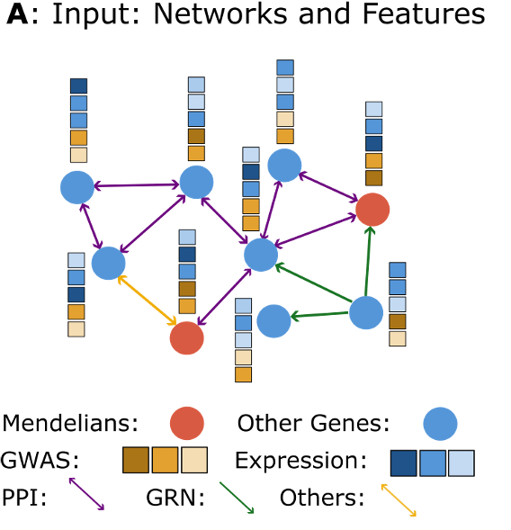
There are several ways in which the input data can be changed using the respective keys in the config file. With Speos, input data can fundamentally be split into three categories: Labels, node features and networks. Labels are shown as nodes of different color, and in Speos nodes are either known positives (usually Mendelian disorder genes) or they are unlabeled genes. The goal is to extract likely positive candidates from the unlabeled genes. The second type are node feautures, which are shown as stacks above the nodes. They consist of disease-specific feauters (from GWAS) and disease unspecific features (median gene expression per tissue). The last data type, the networks, are the connections between the genes. They can have directionality and different types.
Lets go through the most important settings you should know when manipulating input data.
Adjacency Matrices (Networks)
From the default config (excerpt):
1input:
2    adjacency: BioPlex30293T
3    adjacency_field: name
4    adjacency_blacklist: [recon3d, string]
These settings control the adjacency matrices used for construction of the GNN. All settings here are relative to the adjacency definitions provided in speos/adjacencies.json and, if you added some of your own, in extensions/adjacencies.json. By using the settings above, each entry that contains the value “BioPlex30293T” in the field “name” in those two files will be used for the GNN message passing. Standard python string matching in lower case is possible, so just putting “bioplex” will give you both BioPlex networks. You can, however, use any field in the two files for matching. If you want to use all Protein-Protein-Interaction (PPI) networks, set adjacency: ppi and adjacency_field: type. Using adjacency: all will give you all networks that arent explicitely blacklisted. adjacency_blacklist lets you control what should not be used, even if it matches the criteria set above. As you see, recon3d and string are not used, even though they are included in the framework. String was excluded due to the degree distribution, and recon was simply added after all experiments were performed. You can already use it, but since we want Speos to recreate our experiments by default, it is on the blacklist for the time being.
Note that the adjacency matching works also for multiple keywords, for example, the following setting:
1input:
2    adjacency: [bioplex, evo]
3    adjacency_field: [name, type]
loads all adjacencies that match the string “bioplex” in the field “name” or the string “evo” in the field “type”. Thus, this setting loads three adjacencies, Bioplex 3.0 HEK293T, BioPlex 3.0 HCT116 and Hetionet Covaries. This can be extended indefinitely with more keywords, such as:
1input:
2    adjacency: [bioplex, huri, evo]
3    adjacency_field: [name, name,  type]
Which additionally loads HuRI.
Node Features
From the default config (excerpt):
1input:
2    gwas_mappings: ./speos/mapping.json
3    tag: Immune_Dysregulation
4    field: ground_truth
5    use_gwas: True                        # if gwas features should be used
6    use_expression: True                  # if tissue wise gene expression values should be used
7    use_embeddings: False                 # if the embeddings obtained from node2vec should be concatenated to the input vectors (laoded from embedding_path)
8    embedding_path: ./data/misc/walking_all.output
gwas_mappings controls which GWAS trait is mapped to which set of Mendelian disorder genes. tag and field control which gwas-to-disease mappings should be used for the run. In this case, all GWAS traits that are mapped to the Mendelian disorder genes matching “Immune_Dysregulation” are used as input. Changing this field to “Cardiovascular” will make Speos use different positive labels and different, matching GWAS traits! use_gwas and use_expression are boolean flags that control if the respective type of input features are used for this run. This is useful for ablation studies. use_embeddings lets you include the pre-trained node embedding vectors using Node2Vec. You can also train them yourself and add them with the key embedding_path.
This should give you a good overview on how to customize the input data of your runs.
Model Settings
Most of Speos’ usefulness is that it lets you pick, choose and configure across a wide range of models, including GNNs, MLPs and non-neural models. To accomplish that, the config file hosts an array of settings that can be tweaked to fit your needs. Here, we will walk through the most important of them.
The general model architecture is shown here in a:
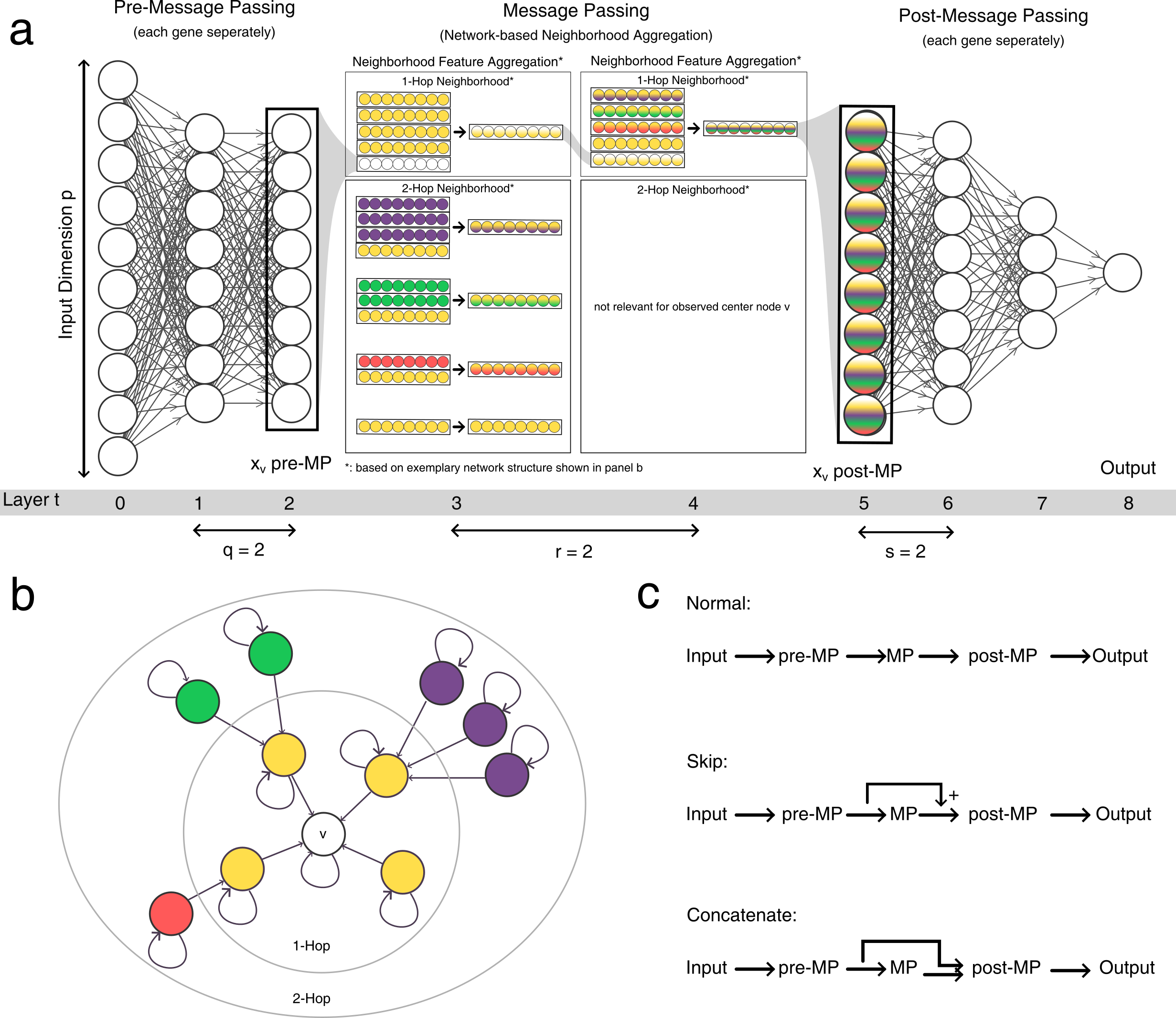
We can not only modulate the depth of the modules q, r and s, we can also modulate the way the features are aggregated in the message passing module by choosing graph convolution layers. Furthermore, we can modify the width, i.e. the hidden dimension of the modules. Furthermore, we can choose different information flows (as shown in c). Finally, we can choose to not use graph convolutions at all, or ditch the neural network approach alltogether and use logistic regression or random forest models instead!
Let’s walk through the relevant settings and see what they mean.
General
From the default config (excerpt):
1model:
2    model: SimpleModel            # SimpleModel, LogisticRegressionModel, RandomForestModel, SupportVectorModel or AdversarialModel (untested)
3    architecture: GeneNetwork     # only relevant for SimpleModel and AdversarialModel, is automatically updated to RelationalGeneNetwork if more than one network is used
4    args: []                      # args passed to model initialization
5    kwargs: {}                    # kwargs passed to model initialization
First, the model keyword changes the highest-order model abstraction. All neural models (GNNs, MLPs etc) that have to be trained using gradient descent fall into the SimpleModel category.
On top of that, you also have LogisticRegressionModel, RandomForestModel and SupportVectorModel for which the respective scikit-learn models will be created and trained. Most of the settings we will be discussing here are only relevant for SimpleModel.
architecture is only relevant for model: SimpleModel and defines the specific neural network architecture that we will use. All our experiments use the GeneNetwork architecture, which is automatically changed to RelationalGeneNetwork if we use more than one adjacency matrix.
If you want to implement your own neural network from scratch, this is where you’d insert your model. args and kwargs lets you define additional arguments and keyword arguments for the initialization of the model.
Pre- and Post-Message Passing
Lets first look at the pre-message passing and post-message passing. These neural network modules transform the input space into the latent space and perform gene-level pattern recognition (pre-message passing) or transform the latent space into the output space and perform the classification (post-message passing.) They are built from fully connected neural networks which can be configured in depth, width and a few other features.
From the default config (excerpt):
1model:
2    pre_mp:
3        dim: 50
4        n_layers: 5        # resulting number of layers will be n_layers + 1 for the input layer
5        act:  elu
6    post_mp:
7        dim: 50
8        n_layers: 5        # resulting number of layers will be n_layers + 2 for the output layer
9        act:  elu
dim lets you control the hidden dimension across the layers. while n_layers controls the number of layers. if you set it to 0, pre_mp will only contain one mandatory layer fitting the input space to the GNNs hidden space and post_mp will contain only two mandatory layers fitting the hidden space to the output space.
act lets you defince the activation function (nonlinearity). At the moment, only elu and relu are implemented, but if you would like to use other activation functions, do not hesitate to send us a feature request via GitHub Issues <https://github.com/fratajcz/speos/issues>.
Message Passing (GNN)
Now, lets look at the message passing (GNN) settings:
From the default config (excerpt):
1model:
2    mp:
3        type: gcn
4        dim: 50
5        n_layers: 2
6        normalize: instance   # instance, graph, layer
7        kwargs: {}
This is where you can define which GNN layer you want to use, how many of them, and how the normalization should look like.
First, type can take 13 different forms: “gcn”, “sgcn”, “sage”, “tag”, “fac”, “transformer”, “cheb”, “gcn2”, “gin”, “gat” and the relational layers “rgcn”, “rgat” and “film”.
To see how they work in detail, check the overview from PyTorch Geometric with the respective publications. Most of them should be easy to identify.
If you feel like that is not enough and you would like to test a different layer, you can specify every layer that is implemented in pyg_nn and refer to it by its class name (case sensitive).
For example, if you’d like to use GraphConv instead of GCN, then use type: GraphConv and Speos will try to dynamically import and use that layer.
dim and n_layers lets you define the width and depth of the GNN. normalize lets you pick either instance, graph or layer normalization applied after each GNN layer. To see their differences, check here.
kwargs lets you pass additional keyword arguments for to the layer initialization. Simple keyword arguments can be specified by passing in key, value pairs:
1model:
2    mp:
3        type: gcn
4        kwargs: {aggr: max}
This little snipped changes the neighborhood aggregation keyword of the GCN layer from mean (the default) to max. However, Speos also supports the passing of more sophisitcated keywords, such as classes imported from either pyg_nn or (PyTorch) nn.
For example, the FiLM layer from PyTorch Geometric by default uses a single linear layer of shape (hidden_dim, 2 * hidden_dim) for it’s feature wise linear modulation. by using its nn keyword, we can input arbitrary other neural networks, like the PyTorch Geometric MLP class with two layers (one with shape (hidden_dim, 1.5 * hidden_dim) and one with shape (1.5 *hidden_dim, 2 * hidden_dim)):
1model:
2    mp:
3        type: film
4        kwargs:
5            nn: pyg_nn.models.MLP([50,75,100])
Another example on how to achieve the same is to build a Sequential Model right out of its (PyTorch) nn building blocks:
 1model:
 2    mp:
 3        type: film
 4        kwargs:
 5            nn: nn.Sequential(
 6                nn.Linear(50,75),
 7                nn.ReLU(),
 8                nn.Linear(75,100),
 9                nn.ReLU()
10                )
Be aware that for now, all classes imported and created this way have to originate in pyg_nn or (PyTorch) nn. If you would like to use other classes which can not be imported from these two sources, make sure to send us a feature request via GitHub Issues.
Advanced
There are a few other model settings which might be worthwile introducing.
From the default config (excerpt):
1model:
2    loss: bce
3    skip_mp: False    # boolean, use skip connections that skip message passing
4    concat_after_mp: False  # boolean, concatenate pre_mp and mp features and feed them both into post_mp
loss manages which loss will be used during training. All our experiments use binary cross entropy (“bce”), but feel free experimenting with mean squared error (“mse”), LambdaLoss (“lambdaloss”), NeuralNDCG (“neuralndcg”), ApproxNDCG (“approxndcg”), UPU (“upu”) and NNPU (“nnpu”) loss.
We have not found this to make a big difference, but it might in your case.
skip_mp will add the output of pre-message passing to the output of the message passing before feeding it into the post-message passing, while concat_after_mp will concatenate the latent feature matrices instead of adding them (as shown above in C).
This will let information bypass the GNN which might be helpful for some layers and architectures.